TLDR;
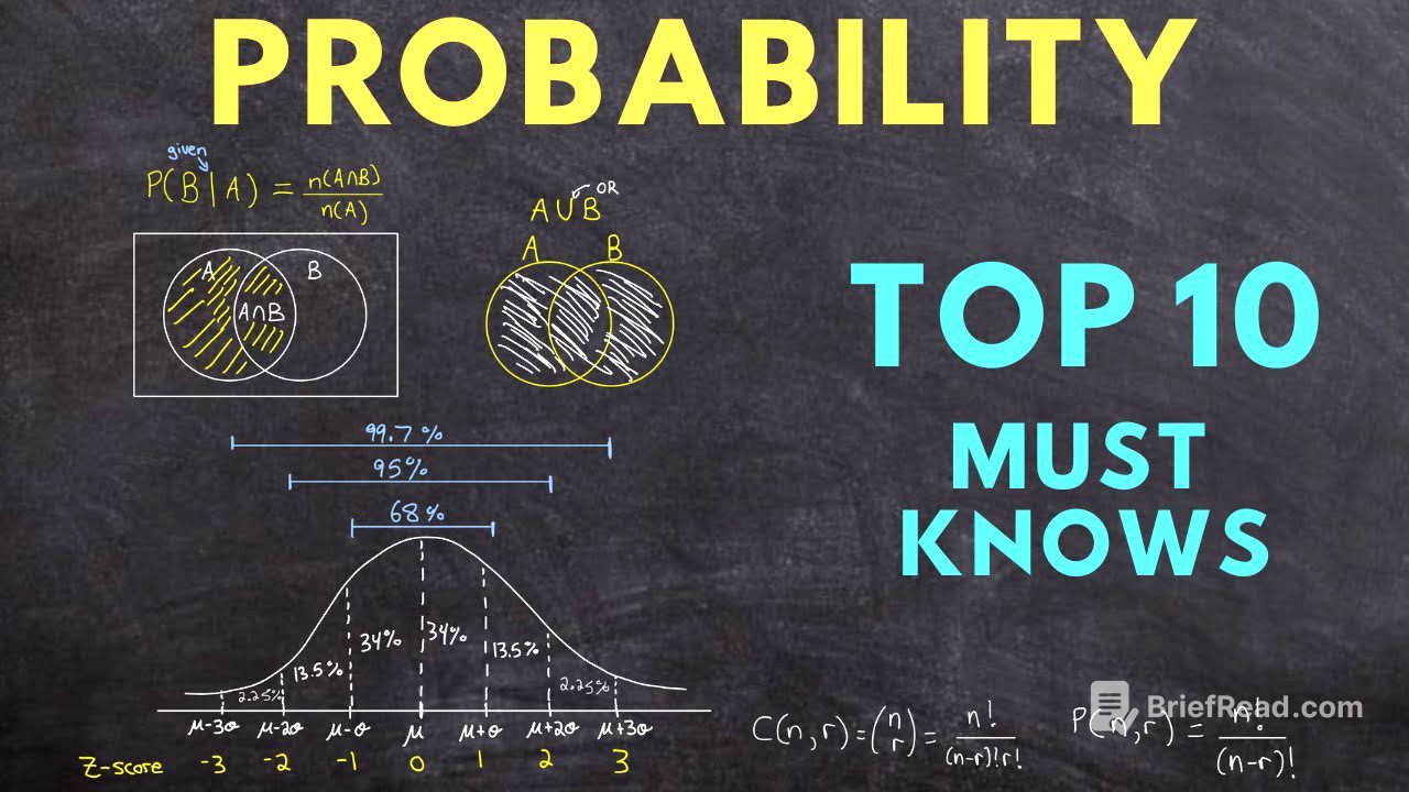
This video provides a comprehensive overview of the top 10 essential concepts in probability, including experimental and theoretical probability, set theory applications, conditional probability, multiplication law, permutations, combinations, continuous and discrete probability distributions like binomial and geometric. It explains key formulas, provides examples, and clarifies the differences between various probability types, offering a solid foundation for understanding and solving probability problems.
- Experimental vs. Theoretical Probability
- Set Theory in Probability (Intersection, Union)
- Conditional Probability and the Multiplication Law
- Permutations and Combinations
- Continuous (Normal Distribution) and Discrete (Binomial, Geometric) Probability Distributions
Experimental Probability [0:00]
Experimental probability is determined through conducting experiments and observing outcomes. It's calculated by dividing the number of times an event occurs by the total number of trials. For example, flipping a coin 10 times and observing 3 tails results in an experimental probability of 3/10 or 30% for flipping tails. Increasing the number of trials generally brings the experimental probability closer to the theoretical probability.
Theoretical Probability [3:01]
Theoretical probability uses reasoning and math to predict the likelihood of an event, calculated by dividing the number of favorable outcomes by the total number of possible outcomes. Examples include calculating the probability of rolling a specific number on a die, drawing a certain card from a deck, or picking a colored marble from a bag. The probability of an event not occurring is 1 minus the probability of it occurring.
Probability Using Sets [7:58]
Probability using sets involves understanding the intersection and union of sets within a sample space, often visualized using Venn diagrams. The intersection (A and B) includes elements common to both sets, while the union (A or B) includes elements in either or both sets. The probability of A or B is calculated as P(A) + P(B) - P(A and B) to avoid double-counting elements in the intersection.
Conditional Probability [14:07]
Conditional probability is the likelihood of an event occurring given that another event has already occurred. It's calculated using the formula P(B|A) = P(A and B) / P(A), where P(B|A) is the probability of event B given event A. The sample space is reduced to only include the outcomes where event A has occurred. For example, the probability that a respondent likes school given they are female.
Multiplication Law [17:19]
The multiplication law calculates the probability of multiple events happening in sequence. For independent events, the probability of both events occurring is the product of their individual probabilities: P(A and B) = P(A) * P(B). For dependent events, where one event affects the other, the formula is P(A and B) = P(A) * P(B|A), incorporating conditional probability.
Permutations [22:11]
Permutations refer to ordered arrangements of objects. The number of permutations of n distinct objects is n!. When arranging r items from a set of n, the formula is n! / (n-r)!. This concept is used in probability to calculate the number of possible ordered outcomes, such as the number of ways people can finish in a race or the probability of guessing a correct passcode.
Combinations [27:37]
Combinations are selections of objects where order doesn't matter. The number of combinations of n items taken r at a time is calculated as n! / (r!(n-r)!). This is used to find the number of possible groups that can be formed from a larger set, such as the number of teams that can be made from a group of people, or to calculate probabilities involving unordered selections.
Continuous Probability Distributions [31:56]
Continuous probability distributions model probabilities of continuous random variables, focusing on normal distributions. A probability density function (PDF) models the probabilities of outcomes, with the total area under the curve equaling 1. Key properties include the mean being at the highest peak, and specific percentages of data falling within standard deviations of the mean (68% within one, 95% within two, 99.7% within three). Z-scores and z-score tables are used to find probabilities relative to the standard normal distribution (mean of 0, standard deviation of 1).
Binomial Probability Distribution [40:11]
A binomial probability distribution describes the probability of successes in an experiment with a fixed number of independent trials, each having only two outcomes: success or failure. The probability of k successes in n trials is calculated using the formula: P(K=k) = (n choose k) * p^k * (1-p)^(n-k), where p is the probability of success. This distribution is discrete, and the expected value (mean) is n*p.
Geometric Probability Distribution [46:01]
A geometric probability distribution models the probability of the number of trials needed to achieve the first success in an experiment. The formula for the probability of the first success occurring on trial k is P(X=k) = (1-p)^(k-1) * p, where p is the probability of success. The expected waiting time before the first success is 1/p.