TLDR;
This lecture introduces the integrated course on quantum theory, emphasizing its conceptual difficulty compared to classical mechanics. It highlights the need for a new mathematical framework to account for phenomena like the discrete spectrum of measurement results, the irreducible impact of measurements on quantum states, and the probabilistic nature of predictions. The lecture culminates in presenting the five core axioms of quantum mechanics, setting the stage for the course's exploration of the functional analysis required to understand and apply these axioms.
- Quantum mechanics is conceptually difficult because it differs significantly from our everyday experiences and classical mechanics.
- Quantum mechanics needs to account for discrete measurement results, the impact of measurements on the state of a quantum system, and the probabilistic nature of predictions.
- The five axioms of quantum mechanics are introduced: the association of a complex Hilbert space with every quantum system, the definition of states as positive trace-class linear maps, the representation of observables as self-adjoint linear maps, the unitary dynamics governing time evolution, and the projective dynamics describing state changes upon measurement.
Introduction to Quantum Theory [0:08]
The lecture begins by welcoming students to the quantum theory course, an integrated course taught by an experimentalist and a theorist. While the instructors strive for harmony between the experimental and theoretical aspects, they acknowledge that complete harmony would sacrifice the content of each. Quantum mechanics is presented as a challenging subject, differing significantly from classical mechanics and electromagnetism in its conceptual underpinnings. Unlike classical mechanics, which aligns with our intuitive understanding of the world, quantum mechanics often contradicts it.
The Failure of Classical Mechanics [0:55]
Classical mechanics works well for large masses, but it is fundamentally incorrect for smaller objects like electrons. The double-slit experiment demonstrates that electrons do not follow defined trajectories, challenging the core principles of classical mechanics. This effect, while more difficult to observe, also applies to larger objects like whales, indicating the universal nature of quantum mechanics. The lecture emphasizes that classical mechanics is not just inaccurate for electrons but fundamentally wrong for all objects, regardless of size.
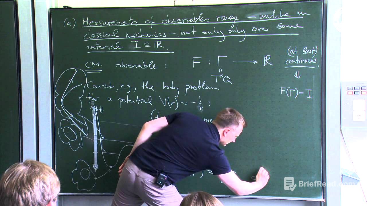
Desiderata for Quantum Mechanics [3:43]
The lecture transitions to outlining what quantum mechanics needs to account for, avoiding the term "explain." The first point is that measurements of observables range over a spectrum, unlike in classical mechanics, where they range over an interval. In classical mechanics, observables are continuous maps from phase space to real numbers, resulting in continuous intervals of possible values. However, quantum mechanics reveals discrete energy levels, as seen in the hydrogen atom, which classical mechanics cannot explain.
Discrete Spectra and New Mathematics [12:31]
Measurements of the hydrogen atom's energy levels reveal discrete values, contrasting with the continuous range predicted by classical mechanics. The energy levels are defined by the formula -13.6 eV / n^2, where n is a positive integer. This discrete nature necessitates new mathematics to define observables that allow for such spectra of measurement results. The lecture introduces the concept of a quantum observable, denoted as 'a', which is associated with a set of possible measurement results consisting of discrete and continuous parts.
Examples of Quantum Systems [19:46]
Various examples illustrate the diverse spectra of observables in quantum systems. The hydrogen atom exhibits a discrete spectrum with an accumulation point at zero, followed by a continuous spectrum. The quantum harmonic oscillator demonstrates equidistant energy levels. In contrast, the position observable for the same harmonic oscillator has a continuous spectrum. A simple model of a solid body shows bands of possible energy levels, further highlighting the departure from classical mechanics.
Self-Adjoint Linear Maps and Observables [26:10]
Self-adjoint linear maps on a complex Hilbert space are introduced as a suitable structure to model observables in quantum mechanics. This means that quantum observables, such as energy (H) and position (Q), will be represented by these mathematical entities. The lecture emphasizes that these self-adjoint linear maps are used differently than classical observables, encoding information about measurement in a non-classical way.
The Irreducible Impact of Measurement [28:17]
Quantum mechanics must account for the irreducible impact of each measurement on the state of a quantum system. Unlike classical mechanics, where measurements do not alter the system's state, quantum measurements fundamentally change the state. The Stern-Gerlach experiment is presented as a crucial example, demonstrating that silver atoms passing through an inhomogeneous magnetic field are deflected in only two directions, not a continuous range as predicted classically.
Successive Stern-Gerlach Apparatuses [36:05]
The lecture explores the implications of the Stern-Gerlach experiment through a series of successive measurements. By blocking one of the outputs and sending the remaining atoms through another Stern-Gerlach apparatus, the experiment reveals that measurements alter the state of the system. Specifically, filtering atoms with a Z-up orientation and then measuring their X orientation results in a 50/50 split between X-up and X-down. However, subsequent measurement in the Z direction reveals that Z-down atoms reappear, demonstrating that the X measurement has changed the state of the system.
Measurements Change the State [42:55]
The key conclusion drawn from the Stern-Gerlach experiment is that measurements change the state of a quantum system. This is not due to experimental imprecision but is a fundamental aspect of quantum mechanics. The act of looking or measuring alters the system, meaning the state before the measurement is not the same as the state after.
Probabilistic Predictions in Quantum Mechanics [48:06]
Even with complete knowledge of a quantum system's state, the only prediction one can make for the measurement of an observable is the probability of obtaining a result within a certain range. This probability is calculable and denoted by µ, representing a measure on the real numbers. The lecture introduces the concept of Borel measurable sets and measure theory, which are essential for dealing with both discrete and continuous spectra in quantum mechanics.
Limitations of Prediction and Impact of Measurement [56:56]
Quantum mechanics limits our ability to predict the concrete outcome of an isolated measurement. Furthermore, the precise impact of a measurement on the state of the system depends on the concretely measured value. This means that the state changes differently depending on the outcome, making it impossible to predict beforehand how the measurement will alter the system's state.
A Suitable Theory for Quantum Mechanics [1:02:50]
The lecture concludes the overview by stating that a suitable theory accommodating all known experimental facts has been developed roughly from 1900 to 1927. Key figures in this development include Planck, Bohr, Schrödinger, Heisenberg, Dirac, and von Neumann. Von Neumann's work on functional analysis is highlighted as essential for providing a proper mathematical foundation for quantum mechanics. The course will focus on developing the necessary functional analysis to understand quantum mechanics properly.
Axiom 1: Complex Hilbert Space [1:13:26]
The lecture transitions to presenting the axioms of quantum mechanics, starting with the first axiom: with every quantum system, there is associated a complex Hilbert space. A Hilbert space is defined as a tuple consisting of a set H, an operation plus, an operation S multiplication, and a sesquilinear inner product. The states of the system are all positive trace-class linear maps row from the Hilbert space into itself, with the trace of this map equaling one.
Pure vs. Mixed States [1:17:36]
The lecture clarifies a common misconception in the literature, stating that normalized elements of the Hilbert space are not the states of the quantum system. Instead, states are positive trace-class linear maps. A state is called pure if there exists a sigh in the Hilbert space such that the row can be expressed entirely in terms of the S. If a state is not pure, it is called a mixed state.
Definitions: Complex Hilbert Space [1:21:39]
The lecture provides definitions for the components of a complex Hilbert space. H is a set, plus is a map that takes two elements of H back into H, and times is a map that takes a complex number and an element of H back to H. These operations must satisfy the vector space axioms. The sesquilinear inner product is a map that takes two elements of H and produces a complex number, satisfying properties such as the Hermitian property, sesquilinearity, and positivity.
Completeness of Hilbert Space [1:26:42]
In addition to being a complex vector space with a sesquilinear inner product, a Hilbert space must also be complete. Completeness means that if one has a sequence in H that satisfies the Cauchy property, then the sequence converges in H. This property is crucial for many proofs in quantum mechanics.
Linear Maps and Positive Linear Maps [1:35:41]
The lecture defines a linear map as a map A from a domain (which may be a proper subset of the vector space) into the vector space. The lecture focuses on densely defined linear maps, where the domain is a dense subset in the vector space. A positive linear map is a map such that for all s in the domain of A, the inner product of s with A(s) is greater than or equal to zero.
Trace Class Operators [1:39:45]
A linear map A is of trace class if, for any orthonormal basis e_n, the sum of the inner products of e_n with A(e_n) is less than infinity. If this condition is met, the trace of A is defined as this sum. For A to be of trace class, it must be defined on the entire Hilbert space.
Axiom 2: Observables as Self-Adjoint Linear Maps [1:43:11]
The second axiom states that the observables of a quantum system are the self-adjoint linear maps A from a domain (which is dense in H) to H. The lecture emphasizes that the condition of self-adjointness is very subtle and will require significant effort to understand fully.
Definition of Self-Adjointness [1:44:55]
A linear map A is called self-adjoint if it coincides with its adjoint map A*. To coincide, the domains of A and A* must be the same, and A*(s) must be the same as A(s) for all s in the domain. The adjoint A* is defined in two steps: first, by defining its domain, and second, by defining its action.
Defining the Adjoint Map [1:47:17]
The domain of the adjoint A* consists of all elements s in the Hilbert space such that for all alpha in the domain of A, there exists an eer in the Hilbert space such that the inner product of s with A(alpha) equals the inner product of eer with alpha. The action of A* on such a s is defined as eer.
Axiom 3: Probability of Measurement Results [1:52:38]
The third axiom states that the probability that a measurement of an observable A on a system in state row yields a result in the Borel set E is given by the trace of PA(E) * row, where PA is a projection-valued measure associated with the self-adjoint map A. This PA is a map from all possible measurable sets into the bounded linear maps on H.
The Spectral Theorem [1:57:09]
The projection-valued measure PA is associated with a self-adjoint map A according to the spectral theorem. The spectral theorem states that for any self-adjoint operator A, you can find a projection-valued measure PA such that A can be represented as the integral over Lambda of Lambda dPA(Lambda). This is the analog of the diagonalization theorem for symmetric matrices in the infinite-dimensional case.
Axiom 4: Unitary Dynamics [2:00:24]
The fourth axiom describes unitary dynamics, which prevail during time intervals when no measurement occurs. The state row at time T2 is related to the state row at time T1 through the equation row(T2) = U(T2 - T1) * row(T1) * U inverse(T2 - T1), where U(T) is the exponential of -i/h_bar * H * T, and H is the energy observable of the quantum system.
Functions of Self-Adjoint Operators [2:03:13]
The lecture defines the function of a self-adjoint operator as F(A) = integral from -infinity to infinity of F(Lambda) dPA(Lambda), where PA is the projection-valued measure associated with A. This definition is crucial for understanding the unitary dynamics of quantum systems.
Axiom 5: Projective Dynamics (Collapse of the Wave Function) [2:04:19]
The fifth axiom describes projective dynamics, which take place when a measurement is made. The state row after a measurement of an observable A is given by PA(E) * row_before * PA(E) divided by the trace of the numerator, where E is the smallest Borel set in which the actual outcome of the measurement happened to lie. This axiom highlights that the way the state before the measurement is mapped to the new state depends on the actual outcome of the measurement.