TLDR;
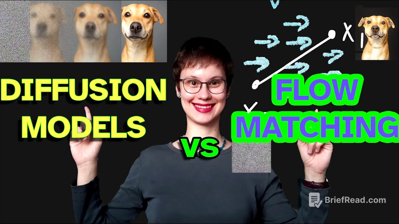
Alright, so this video breaks down the difference between flow-matching and diffusion models, which are both used for generating images. Diffusion models, like Stable Diffusion, were the go-to, but now flow-matching models, such as Flux, are becoming popular. The video explains how diffusion models are trained to reverse noise and generate images, then compares this process step-by-step with flow-matching models to highlight the key differences. Flow matching simplifies the process by using deterministic flows instead of random noise, leading to faster image generation.
- Diffusion models reverse noise through stochastic steps.
- Flow-matching models use deterministic flows for faster image generation.
- Training involves different approaches: noise prediction vs. velocity field prediction.
Difference between Flow-matching and Diffusion [0:00]
The video is all about understanding the shift from diffusion models to flow-matching models in image generation. Diffusion models like Stable Diffusion used to be top-notch, but now flow-matching models like Flux and Stable Diffusion 3 are gaining traction. The video aims to explain what flow matching does differently compared to diffusion, breaking down the training and image generation processes of both.
Training Diffusion Models [1:07]
Diffusion models basically learn to reverse noise. They take a completely noisy image and step-by-step transform it into a realistic image. During training, a real image (X1) is taken from the dataset, and a random time step T (between 0 and 1) is selected. Gaussian noise (epsilon) is added to each pixel of X1 to create a noisy version (XT). The amount of noise is determined by a schedule (BT) that increases with T. The neural network predicts the noise (epsilon hat) added during the forward diffusion. The network is trained using an L2 loss function to match the predicted noise with the actual noise added.
Inference for Diffusion Models [5:45]
To generate images, the trained diffusion model reverses the diffusion process. The formula used for adding noise is rearranged to solve for the clean image. Starting with a completely noisy image (x0), the model predicts the noise present. Using the backward diffusion formula, the predicted noise is subtracted from the image to get a cleaner image (xt+1). This process is done iteratively, removing a bit of noise at a time, because the model has learned to denoise specific amounts of noise at time steps t. The model integrates these small steps over the whole noise schedule from t=0 to t=1, using its prediction at each step to guide the process.
Training Flow-Matching [9:03]
Flow matching simplifies the process by making it deterministic, removing the Gaussian noise term and using an ordinary differential equation (ODE). The model learns the velocity field (V) via a neural network. Velocity is the change in position over time, so knowing the velocity field allows recovery of the trajectory by integrating it over time. To train, a data point (X1) is taken from the image database, and a time step t (between 0 and 1) is sampled. A completely noisy image (X0) is also sampled. XT is generated through linear interpolation of X1 and X0. The ground truth velocity field is computed by subtracting X0 from X1. The neural network predicts V, taking XT and T as input, and is trained using a mean squared error loss between the predicted velocity (V hat) and the ground truth velocity (V).
Inference with Flow-Matching [11:55]
To generate images with a trained flow-matching model, start by generating random noise (X0). The network predicts V, and the ODE is integrated forward in time to arrive at X1. A numerical solver, like adaptive Runge-Kutta, is used for integration. The solver starts at t=0 from pure noise, evaluates V to see which direction to move, and takes adaptive steps until t=1, the final image, is reached. Multiple steps are needed because the model has learned an approximation of the global path, and the velocity might vary along the path. Flow matching needs fewer model calls (5-15) compared to diffusion models, allowing for faster high-quality image generation.
Side-by-Side Comparison [14:02]
Flow matching models replace the randomness of diffusion with a smooth, deterministic flow, simplifying the stochastic differential equation (SDE) to an ordinary differential equation (ODE). For training, a data point, a time step t, and a random noise sample X0 are sampled. Interpolation between the real image and noise is done, and the ground truth velocity is computed. The neural network learns to predict this velocity, unlike diffusion models where the network predicts added noise. A mean squared error loss is used to enforce correct velocity prediction. At inference, the learned velocity field is integrated using a solver, tracing the flow to the final image. Diffusion models undo random noise through stochastic steps, while flow matching models learn a deterministic flow, transporting points from the noise distribution to the data distribution.