TLDR;
This lecture explains the zero-one programming problem and the Balas implicit enumeration algorithm for solving it. It highlights the importance of zero-one programming in decision-making, where variables can only take values of zero or one. The lecture contrasts explicit enumeration (trying all possible solutions) with implicit enumeration (intelligently filtering solutions). It details the pre-processing steps required for the Balas algorithm, including converting the objective function to minimise type with positive coefficients and transforming constraints to a "greater than or equal to zero" form. The lecture walks through an example problem, demonstrating how to apply the algorithm, including concepts like free variables, fixed sets, distance from feasibility, and backtracking.
- Zero-one programming involves variables with values of 0 or 1 for decision-making.
- Balas implicit enumeration algorithm efficiently solves zero-one programming problems.
- Pre-processing steps are crucial for applying the Balas algorithm.
- The algorithm uses concepts like free variables, fixed sets, and distance from feasibility.
- Backtracking is used to explore different solution paths.
Introduction to Zero-One Programming and the Balas Algorithm [0:03]
The lecture introduces the concept of zero-one programming, a critical area in decision-making where variables can only assume the values of zero or one, representing choices like "yes/no" or "true/false". These decisions are crucial as they often lead to a final decision. The lecture uses the example of selecting a cricket team's batting order, where each player's position is determined by a series of zero-one variables. The lecture contrasts two approaches to solving such problems: explicit enumeration, which involves trying all possible combinations, and implicit enumeration, which intelligently filters out combinations that won't lead to an optimal solution. The lecture focuses on the Balas implicit enumeration algorithm.
Problem Statement and the Inefficiency of Explicit Enumeration [2:01]
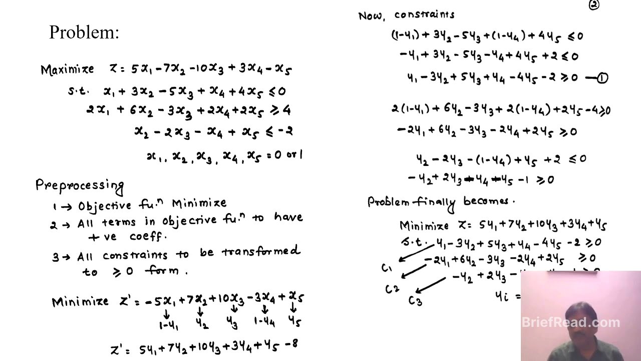
The lecture presents a specific zero-one programming problem with five variables, an objective function to maximise, and three constraints. It explains that solving this problem using explicit enumeration would require testing 2 to the power of 5 (32) combinations. While this is manageable for a small number of variables, the lecture points out that real-world problems often involve thousands of variables, making explicit enumeration impractical due to the enormous number of combinations (2 to the power of 1000 or more) that would need to be evaluated. This highlights the need for more efficient methods like implicit enumeration.
Pre-processing Steps for the Balas Algorithm [4:34]
To prepare the problem for the Balas implicit enumeration algorithm, several pre-processing steps are necessary. First, the objective function must be of the minimise type. Second, all terms in the objective function must have positive coefficients. Third, all constraints must be transformed to a "greater than or equal to zero" form. The lecture emphasises that these steps are not arbitrary but have specific reasons that will become clear as the algorithm is applied.
Transforming the Objective Function [5:52]
The lecture details the process of converting the objective function from maximise to minimise by multiplying it by -1. It then addresses the requirement for positive coefficients. To achieve this, variables with negative coefficients (e.g., x1) are substituted using the formula x1 = 1 - y1. This ensures that the new variable (y1) also takes values of 0 or 1. The lecture explains why simply substituting x1 with -y1 is not suitable, as it could lead to y1 having a value of -1 when x1 is 1, violating the zero-one constraint. To maintain homogeneity, all x variables are converted to y variables, even those with positive coefficients. The constant term resulting from these substitutions can be kept or eliminated from the objective function.
Transforming the Constraints [10:14]
The lecture explains how to transform the constraints to a "greater than or equal to zero" form. This involves substituting the x variables with their corresponding y variables (or 1-y variables where applicable) in each constraint. If a constraint is initially in a "less than or equal to zero" form, all signs are changed to convert it to the desired form. The lecture encourages viewers to perform these transformations themselves to verify the results.
Rationale Behind the Pre-processing Steps [12:18]
The lecture explains the reasons for the pre-processing steps. Having a minimise-type objective function with positive coefficients allows for a clear starting point: a solution of zero (all variables set to zero). If the constraints permit this solution, it is immediately optimal. Converting constraints to a "greater than or equal to zero" form simplifies the evaluation of constraint satisfaction. A positive or zero value indicates satisfaction, while a negative value indicates violation, eliminating the need to compare left-hand and right-hand sides.
Applying the Balas Algorithm: Initial Setup [15:15]
With the pre-processed problem at hand, the lecture begins demonstrating the Balas implicit enumeration algorithm. Initially, all variables are considered "free variables" and are collected in a "free set". The "fixed set" is initially empty, as no variables have been assigned specific values. The algorithm aims to set as many variables as possible to zero, given the minimisation objective.
First Iteration: Evaluating Constraints and Feasibility [17:01]
Assuming all free variables are zero, the lecture calculates the values of the left-hand sides of the constraints (C1, C2, C3). If any constraint is violated (i.e., the value is negative), the algorithm checks the possibility of satisfying that constraint. This involves substituting the free variables with positive coefficients in the violated constraint with a value of one. If, even with these substitutions, the constraint remains violated, the problem has no feasible solution.
Fixing Variables and Calculating Distance from Feasibility [20:35]
If it's possible to satisfy the violated constraints, the algorithm proceeds to fix one of the free variables to one. The lecture introduces the concept of "distance from feasibility," which quantifies how much a constraint is violated. If a constraint is satisfied, the distance is zero; if violated, it's the absolute value of the negative result. The algorithm calculates the total distance from feasibility for each variable fixed to one.
Second Iteration and Backtracking [25:40]
The algorithm selects the variable that results in the minimum total distance from feasibility and fixes it to one. This variable is moved from the free set to the fixed set. The process is repeated: constraints are evaluated, and if violations occur, the possibility of feasibility is checked. Once a feasible solution is found, the value of the objective function (z) is calculated. To find the optimal solution, the algorithm uses backtracking. This involves going back to a previous node and trying a different path (i.e., setting a previously considered variable to zero instead of one).
Modified Preset and Termination of Branches [32:35]
During backtracking, the lecture introduces the concept of a "modified preset". This is a subset of the free set, excluding variables that, if set to one, would cause the objective function to exceed the current minimum known value of z. This helps to prune the search tree. If, at any point, the test for possibility of feasibility indicates that no feasible solution can be obtained along a particular path, that branch is terminated.
Finding the Optimal Solution and Final Substitutions [42:38]
The algorithm continues to explore different branches through backtracking and variable fixing until all possibilities have been exhausted. The feasible solution with the lowest value of z is the optimal solution. Finally, the values of the original x variables are determined by substituting the values of the y variables back into the equations used during pre-processing. The lecture concludes by verifying that the optimal z value obtained using the Balas algorithm matches the z value calculated using the original problem formulation. The lecture encourages viewers to work through the problem themselves to solidify their understanding.