TLDR;
This video demonstrates how to apply dynamic system analysis tools to a real-life biomechanics problem: determining joint reaction forces and moments during the swing phase of walking. It covers setting up the problem in two dimensions, drawing free body diagrams for each segment of the leg (foot, lower leg, and thigh), and applying Newton-Euler equations to solve for unknown forces and moments at the ankle, knee, and hip joints.
- Problem defined in two dimensions (sagittal plane).
- Joint reaction forces and moments calculated at the ankle, knee, and hip during the swing phase of walking.
- Free body diagrams and Newton-Euler equations applied to each segment (foot, lower leg, thigh).
Introduction to Biomechanics Problem [0:00]
The video introduces a biomechanics problem focused on determining joint reaction forces and moments at the ankle, knee, and hip during the swing phase of walking, which is when the trailing foot is off the ground. The problem is simplified to two dimensions, representing movement in the sagittal plane. Kinematic data, including the locations of the ankle, knee, and hip joint centres, along with mass, mass moment of inertia, segment accelerations, angular accelerations, and centre of mass locations for the foot, lower leg, and thigh, are provided.
Visualising the Problem [2:33]
The problem is visualised by mapping the provided coordinates onto a diagram of a person's leg during the swing phase. A coordinate system is established with the measurements given in meters, and the leg is divided into three segments: the foot, the lower leg (shank), and the thigh. Each segment is treated as a rigid body with its own centre of mass. The goal is to determine the joint reaction forces and moments, which are crucial for understanding the loads experienced by bones, cartilage, and tendons during movement.
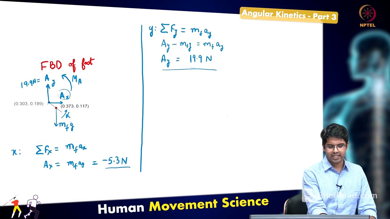
Solving for the Foot Segment [7:20]
To solve the problem, a free body diagram of the foot is drawn first. The forces acting on the foot include its weight (acting downwards) and the reaction forces from the shank at the ankle joint (Ax and Ay). There is also an unknown moment acting on the foot. By applying Newton-Euler equations, the forces in the x and y axes are calculated, as well as the moment at the ankle. The calculations involve summing the forces in each axis and equating them to the mass times acceleration, and summing the moments about the centre of mass and equating it to the moment of inertia times angular acceleration.
Analysing the Lower Leg Segment [19:54]
The analysis moves to the lower leg segment, using the previously calculated reaction forces at the ankle. The free body diagram for the lower leg includes the weight of the segment, reaction forces at the knee joint (Kx and Ky), and the reaction forces from the foot (equal and opposite to those acting on the foot). By applying Newton's third law, the ankle joint forces are used to determine the forces acting on the lower leg. Force balance equations in the x and y axes, as well as the moment balance equation, are used to solve for the unknown forces and moments at the knee joint.
Calculating Forces and Moments at the Knee [23:46]
The force balance equations are set up for the lower leg in both the x and y axes, incorporating the known forces from the ankle joint and the weight of the lower leg segment. These equations are then solved to find the unknown reaction forces at the knee joint (Kx and Ky). Additionally, the moment balance equation is established, considering the moments due to the forces at the ankle and knee joints, as well as any external moments acting on the lower leg. Solving this equation yields the moment at the knee joint (Mk).
Determining Forces and Moments at the Hip [32:20]
Finally, the video provides the solutions for the forces and moments at the hip joint (Hx, Hy, and Mh) without explicitly showing the calculations. It encourages viewers to pause the video and perform the calculations themselves as an exercise. The solutions are given as Hx = 24.6 Newtons, Hy = 101.6 Newtons, and Mh = -11.7 Newton meters.
Conclusion and Applications [33:25]
The video concludes by highlighting the application of linear and angular kinetics tools to solve a biomechanics problem. It emphasises that the principles demonstrated can be extended to various problem statements, including those in three dimensions, although the course focuses on two-dimensional problems. The ability to calculate joint forces and moments has significant implications for sports and clinical applications, as it helps in understanding joint loading and injury potential.